Haar wavelets in Google docs (and R)

Igor recently posted some interesting data, showing the change in temperature over time with 2 different types of fan, or without any cooling. This data exhibits some unusual features: the underlying trend is smooth, over a long timeframe (minutes) but there is also periodic switching between “low” and “high” signal, which is sometimes accompanied by jitter. I’ll first show how to generate some similar data in R, then how we might compute the discrete wavelet transform (DWT) in Google Sheets. Of course, the simplest solution is often the best (unless you work in research…), so check out Igor’s post for a quicker way to filter this data.

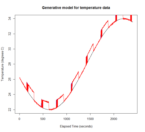
Here I use a sine wave for the overall trend, but this could just as easily be a polynomial or cubic spline. I’m modelling the long-term switching as a deterministic function, although in Igor’s data this appears to be random. I’ve added a small amount of white noise as well as the jitter. I’m assuming a Poisson distribution for the number of time points of jitter following a switching event. A zero-inflated Poisson would be a better model, since jitter only occurs at some of the switches in Igor’s data. Finally, I assemble the four additive components of the signal to produce the red curve in the plot below (the original trend is in black).

t <- 1:2400
trend <- 28 + 6*sin(-0.3 - t/500)
plot.ts(trend, ylab="Temperature (degrees C)", xlab="Elapsed Time (seconds)")
sw <- as.integer(cos(1.7 + t/50) > 0)
lines(trend + sw, col=3)
noise <- rnorm(length(t))/20
lines(trend + sw + noise, col=4)
sw_idx <- which(diff(sw) > 0)
jit_len <- rpois(length(sw_idx), lambda=30)
jit <- rep(0, length(t))
for (i in 1:length(sw_idx)) {
sw_idx2 <- seq(sw_idx[i]+1, to=sw_idx[i] + jit_len[i], by=2)
jit[sw_idx2] <- - 1
}
lines(trend + sw + noise + jit, col=2)

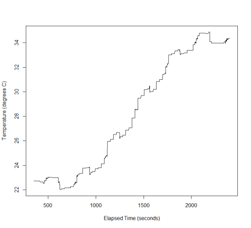
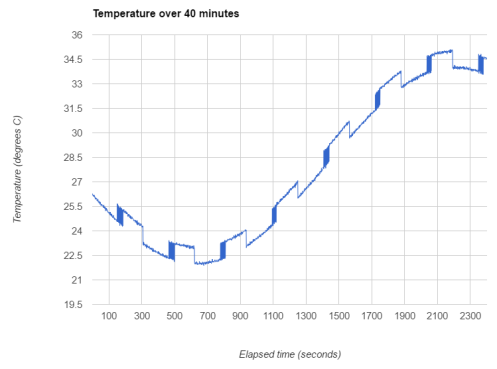
Now that I’ve added the jitter in, I’ll show some ways to filter it out. I’m not using a model-based approach, since ideally this is something one could implement using a spreadsheet. Instead, I threshold the lag 1 difference between successive values to detect the jumps, where jitter is assumed to be two jumps in opposite directions.

temp <- trend + sw + noise + jit
idx1 <- which(diff(temp) > 0.8)
idx2 <- which(diff(temp) < -0.8)
idx3 <- na.omit(match(idx2, idx1+1))
abline(v=idx2[idx3], lty=3, col=3)
filter.temp <- temp
for (i in idx2[idx3]) {
filter.temp[i+1] <- temp[i]
}
plot.ts(filter.temp, ylab="Temperature (degrees C)", xlab="Elapsed Time (seconds)")

Due to the Gaussian noise, a threshold of 0.8 is not guaranteed to catch every instance of jitter. I haven’t set the random seed in this example, so your mileage may vary. Now, to demonstrate how to filter this data in Google Sheets, we could just export a CSV file and upload it. But of course, there is also the R package googlesheets:

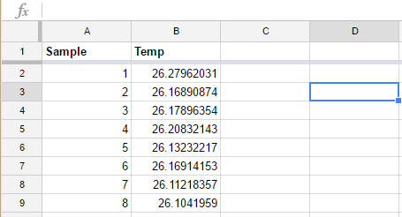
library(googlesheets)
temp_df <- data.frame(cbind(t, temp))
temp_gs <- gs_new(title="Simulated Temperature", verbose = TRUE, input=temp_df)

Sheet "Simulated Temperature" created in Google Drive.
Range affected by the update: "A1:B2401"
Accessing worksheet titled 'Sheet1'.
Sheet successfully identified: "Simulated Temperature"
Accessing worksheet titled 'Sheet1'.
Worksheet "Sheet1" dimensions changed to 2401 x 26.
Worksheet "Sheet1" successfully updated with 4802 new value(s).
Worksheet dimensions: 2401 x 26.
There were 12 warnings (use warnings() to see them)
> warnings()
Warning messages:
1: 'xml2::xml_find_one' is deprecated.
Use 'xml_find_first' instead.
See help("Deprecated")

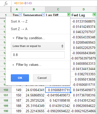
To create the lag 1 difference (and the forward lag), which were named idx1 & idx2 in my R code above, I created 2 new columns with the formulae “B3-B2” & “B2-B3”. Note that the first row of column C is 0 and so is the final row of column D. Filters in Google Sheets are cumulative, which means that we don’t have the same flexibility that we had in R. We can filter by either “Lag Diff <= 0.8” or “Fwd Lag >= -0.8” but not by the intersection of these sets.

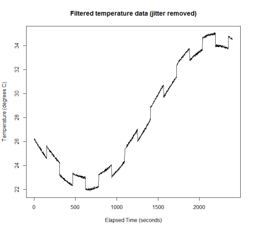
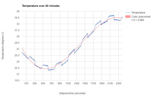
The resulting plot replaces the jitter with a smooth transition between values. In the plot below, I’ve also added a cubic polynomial trend line:

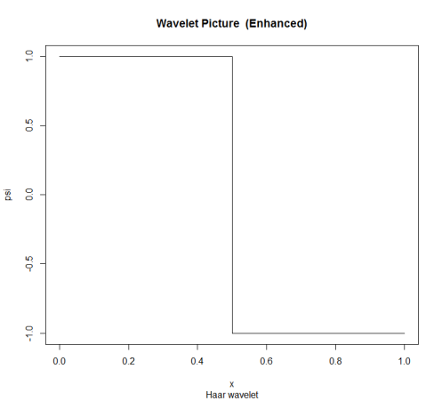
Haar wavelets are very useful functions for changepoint detection in data such as this. There are two excellent reference books on this topic, “Wavelet Methods in Statistics with R” by Guy Nason (part of Springer’s Use R! series) and “A Wavelet Tour of Signal Processing” by Stéphane Mallat. Guy Nason has also created the R package wavethresh, so there is no need to shell out for the MATLAB toolbox.

The discrete wavelet transform (DWT) is only defined for vectors with a length that is a power of 2. Usually we would pad the data to avoid edge effects, but in this case I just truncated it to the last 2048 seconds of temperature measurements.

library(wavethresh)
draw.default(filter.number = 1, family = "DaubExPhase")
temp_wd <- wd(temp, filter.number = 1, family = "DaubExPhase")

Error in wd(temp, filter.number = 1, family = "DaubExPhase") : 
 Data length is not power of two

length(temp) - 2^11 + 1
temp_wd <- wd(temp[353:2400], filter.number = 1, family = "DaubExPhase")
plot(temp_wd)

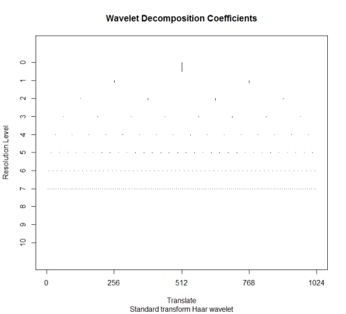
The DWT is a multiscale transform of the data. The Haar wavelet coefficients correspond to the locations of jumps in the data at various resolutions. We have 2^11 time points, so there are 11 resolution levels. Section 2.1 of Nason (2008) describes the DWT algorithm step by step. The complexity of this transform is O(N) and in the case of Haar wavelets it is simple enough to perform in a spreadsheet. At level 10 (the finest resolution), there are 1024 detail coefficients, also known as “mother wavelet” coefficients. Computing this is a little tricky, since we want to subtract the values with even-numbered indices from their preceding values:

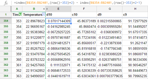
So the first value is B355 – B354, the second is B357 – B356, and so on. Column F contains the coarsening or smoothed coefficients: B355 + B354, B357 + B356, etc. Column G is the next level of resolution: now we take the difference of the smoothed coefficients, so that G354 =  F355 – F354. At each level of resolution, we have half as many coefficients as the previous level: 1024 at level 10, 512 at level 9, and so on. At level 0, we end up with only a single coefficient. Of course, there is no need to compute these by hand when we can just import the data into R, but sometimes it can be beneficial to step through an algorithm in a spreadsheet to understand what it is doing at each iteration.

The point of all of this is that we can filter out noise in our data by shrinking the wavelet coefficients. As a crude example, we can just threshold out any coefficient less than 0.7:

temp_thresh <- threshold(temp_wd, verbose=TRUE, policy="manual", value=0.7)
temp_wr <- wr(temp_thresh)
plot.ts(temp_wr, ylab="Temperature (degrees C)", xlab="Elapsed Time (seconds)")

threshold.wd:
Argument checking
Manual policy
Level:  3  there are  0  zeroes
Level:  4  there are  1  zeroes
Level:  5  there are  9  zeroes
Level:  6  there are  49  zeroes
Level:  7  there are  119  zeroes
Level:  8  there are  251  zeroes
Level:  9  there are  510  zeroes
Level:  10  there are  973  zeroes